Subject: Digital photo of ‘Monck Provincial Park Rock’ on Rockwall.
Tool Used: Colour Pixel Plotter (CPP) and Photo Viewer/editors.
Method: Using Colour Pixel Plotter to ‘construct’ the pictograph image by selective colours
For this pictograph study, our goal is to dissect the entire object to its individual colour components. Where colour is faded, deteriorated, peeled-off or missing, there should be some means of ‘reconstructing’ these affected areas. To this end, CPP will load each pixel’s RGB value into a table with its x/y coordinates; and will plot only the ‘selected’ ones on a uniform background (default is white) at its original x/y position. The pixel ‘selection’ is defined by the user in terms of RGB triplets in a formula-like format. Depending on the actual needs and on individual photo bases, the user can construct a ‘photo’ with one or many formulae as well as which part of the photo to be plotted.
The separation of colours and plotting them either individually or in combinations should allow the scientist to study the following :
- the sequence of colour applied – such as background colour, or over-painting
- whether or not the colour pigment is layered (with some binding agent) or chalk-like
- the surface(rock) colours and texture – given sufficient details
- the component objects may show different colour brightness – may be by different time/creator
- the possibility of part of rock or patch of ‘paint’ (with colours) peeled-off to aid peel search
- the entire pictograph may be a 3-dimensional object and should be studied in sections
- the colours and potential fragments (both paint and rock) that may be found when evacuating soil below
Our Study Plan:
- Study the photo image using a photo viewer/editor (Paint.net and Gimp in this case)
- Load the photo into CPP system
- Define Colour formula for the photo
- Plot by colours to seek outlines of objects – and sequences of colours applied (if any)
- Refine colour formula for better or more detailed coverage
- Observe and analyse differences between objects for component colours and textures
- Summarize findings and define future study plan
Journal of plots from the study
1. Original Photo
The original photo from Monck Park rock, observed using 100% zoom : 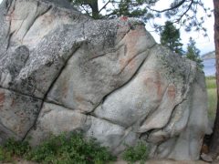
- Colours of interests (RGB values) are :
- Red : Range from bright, washed-out, to dark
- Clay : Appears as possible background for the Red
- Purple : Red with purple tinge – some appear ‘seeping-out’ from dark dots
CPP processing :
- The photo is loaded into CPP with filename ‘monck_a_picto’
- The photo is used in CPP to define ‘colours’ for later used
2. Select the Brightest Red from the photo
Using Colour Search : 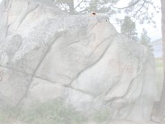
- ‘monck_a_picto’ Table(photo) selected
- ‘monck_a_picto_red-100_180_a’ colour selected
- Colours are defined using CPP Find Colour Menu
- The specification :
- R(100-180)
- R:G ( ( RED * 0.800 ) > GREEN )
- R:B ( ( RED * 0.550 ) > BLUE )
- G:B ( GREEN > BLUE )
- The composite shows where the red pixels are found
3. Select Common Red from the photo (Red b)
Using Colour Search : 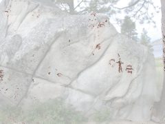
- ‘monck_a_picto_red-100_180_b’ colour selected
- Colours are defined using CPP Find Colour Menu
- The specification :
- R(100-180)
- R:G ( ( RED * 0.850 ) > GREEN )
- R:B ( ( RED * 0.850 ) > BLUE )
- G:B ( GREEN > BLUE )
- The composite shows where the ‘averaged’ red pixels are found
4. Select Clay Colour from the photo
Using Colour Search : 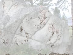
- ‘monck_a_picto_clay_155_220’ colour selected
- The colour were defined using CPP Find Colour Menu
- The specification :
- R(155 – 220) G(140 – 220) B(120 – 200)
- R:G (((RED * 0.98) > GREEN) and ((RED – GREEN) < 15))
- R:B ( ( RED * 0.90 ) > BLUE )
- G:B ( GREEN > BLUE )
- The composite shows where the clay pixels are found
- Noticed that clay actully ‘outlines’ some red components
5. Select Clay and Red_b
Using Colour Search – with two colours – and a partial zone search : 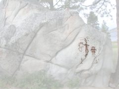
- ‘monck_a_picto_clay_155_220’ colour selected
- ‘monck_a_picto_red-100_180_b’ colour selected
Only the following part of the photo are being searched/plotted :
- Zone specification :
- Width : 1300-1700 (pixels’ x coordinates)
- Height : 600-1100 (pixels’ y coordinates)
- The composite shows where the combined pixels are found
- Notice that ‘figures’ are not quite full of pixels
6. Select Clay and Red_c
Using Colour Search – with two colours : 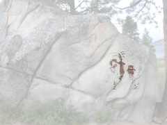
- ‘monck_a_picto_clay_155_220’ colour selected
- ‘monck_a_picto_red-100_180_c’ colour selected
- The ‘red-100_180_c’ specification :
- R(100 – 180)
- R:G ( ( RED * 0.950 ) > GREEN )
- R:B ( ( RED * 0.850) > BLUE )
- G:B ( abs(GREEN – BLUE) < 20 )
- The composite shows where the combined pixels are found
- Notice that ‘figures’ are ‘fuller’
7. Select Red_c Plot
Using Colour Search – modified red_100_180 : 
- ‘monck_a_picto_red-100_180_c’ colour selected
- The ‘red-100_180_c’ specification :
- R(100 – 180)
- R:G ( ( RED * 0.950 ) > GREEN )
- R:B ( ( RED * 0.850) > BLUE )
- G:B ( abs(GREEN – BLUE) < 20 )
- The plot shows where the combined pixels are found
- The selected pixels with its original colours on white
8. Select all defined colours for this photo
Using Colour Search – with all colours : 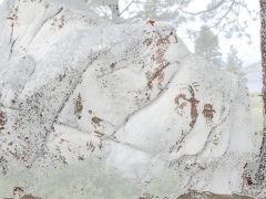
- ‘monck_a_picto_black_027_067’ colour selected
- ‘monck_a_picto_clay_100_220’ colour selected
- ‘monck_a_picto_purple_070_120’ colour selected
- ‘monck_a_picto_red_060_100’ colour selected
- ‘monck_a_picto_red_100_180_a’ colour selected
- ‘monck_a_picto_red_100_180_c’ colour selected
- The composite shows where the combined pixels are found
- Noticed that the left side shows lots of pixels but no ‘pictos’
9. Select all red/clay colours defined for this photo
Using Colour Search – with ‘combined’ red and clay colours 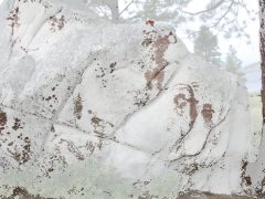
- ‘monck_a_picto_clay_100_200’ colour selected
- ‘monck_a_picto_red_060_200’ colour selected
- The composite shows where the combined pixels are found
- Noticed that picto(s) seems quite well-defined
Based on this plot, the pictograph can be ‘zoned’ for future study :
- Zone 1 : x(0-700), y(0-400) ———- Zone 2 : x(0-600), y(600-900)
- Zone 3 : x(0-400), y(800-1300) —— Zone 4 : x(400-1000), y(400-1000)
- Zone 5 : x(400-1000), y(9500-1300) – Zone 6 : x(1000-1400), y(150-900)
- Zone 7 : x(1300-1800), y(600-1400) – Zone 8 : x(1800-2048), y(1300-1536)