The Anatomy Of Ancient Rock Art: True Colour Analysis Using A Prototype Colour Pixel Plotter

Introduction

Subject: Digital photographs of prehistoric rock wall/cave paintings.

Concept: As stable inorganic compounds, common pigments like red ochre and charcoal preserve their colours. The visibility of their coarse scattered particles in high resolution digital photographic images permits anatomical separation of pictograph elements and palimpsest layers.

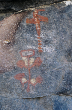
Method: Plotting the position and RGB (red, green, blue) values of each pixel in a pictograph allows precise separation of pictograph elements. Red ochre may include different reds in different elements, or in a palimpsest in one element. When background settings (rock itself or other elements) are removed for clarification, these reds are separable and analyzed on white or neutral backgrounds. The background setting of the rock itself can also be highlighted to show a reverse view of the whole pictograph. A prototype software program was used on an actual Baja California pictograph of a ‘flower’ to anatomically dissect and reassemble its elements.

Based on this simple approach, a prototype software program was developed, and a rock painting ‘Wall Flower’ was used as the subject. The purpose was to determine the utility and relevance of such an application to the study of Wall Paintings.

Test Case

1. Original Photo – Set up the plot database table
   • Preparatory work:
     • The original photo is in ‘jpeg’ format, and the prototype handles ‘png’ only
     • Convert from ‘jpeg’ to ‘png’ using ‘XnView’ (a freeware viewer and converter)
     • All pixels are extracted using prototype function and stored as a text file
     • Photo pixels are then loaded into a database table
   • Photo Size: 1287X1940 pixels (about 2.5 million – 2,496,780 dots)
   • Features: Red Cross with Cream fills
   • Features: Red Flowers with Cream centers
   • The two reds are quite different
2. Search for ‘Cross and Flower’ from the databas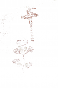e table
   • Preparatory work:
     • The colours are selected by using a ‘colour picker’ from a graphics application
     • Softwares tried: Adobe Photoshop, Gimp, and Paint.net
     • The colours are specified in the Test Run using Gimp
     • There are at least 6 different readings (points) taken for each colour to form the ‘Range’
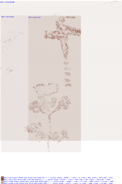
   • Select red for flower: RED(144-162) GREEN(102-125) BLUE(90-111)
   • Select cream for flower: RED(193-210) GREEN(179-194) BLUE(159-189)
   • Select red for cross: RED(137-160) GREEN(74-94) BLUE(53-83)
   • Select cream for cross: RED(193-212) GREEN(174-190) BLUE(161-192)
   • The entire photo is being ‘searched’, partial selection (Width/Height Range) not used
   • The selections are plotted on a white background

3. Visual Report – to refine search colour’s range and parameter

   • Preparatory work:
     • This function evolved during the test case run
     • A quick ‘visual’ report is displayed, so a different ‘range’ can be quickly tried
     • The ‘shading box’ turns out nicely and helpful (based on transparencies of the search colours)
   • This report is plotted on top of the selections
   • The overlays (shadows) draw the boundary of the x,y location of the pixels
   • The text is at the bottom from right – the picture can be shown on bigger window (by clicking on it)
   • Each colour search will have the search parameter, number of pixels found, and the x,y limits
   • Note that we can combine two cream colours as a single specification

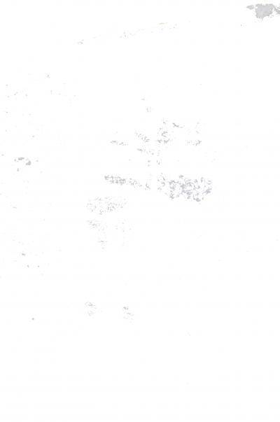
4. A Different View: Plot only black and grey pixels of the photo

   • Preparatory work:
     • The colours are selected by using ‘colour picker’ from the graphics application
     • The DB Table utility lists the most frequent entry by RGB triplet
     • Test and combine finally to two groups (black and grey)
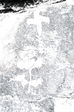
   • This plot searches for the most frequently-appearing colours (background colours)
   • In this instance, most of them are black and greys
   • It is assumed to be the rock surface’s colour
   • The plot actually shows a kind of negative image of the features
   • Note that some are actually inside the features themselves
   • Note also on the lower right there is a patch of something that is actually more blueish

5. New Feature Found – Is the ‘white’ partially covered by the ‘Cross’ also a feature ?

   • Preparatory work:
     • Observing the photo, there looks to be a ‘white’ feature overlayed by the ‘cross’
     • The colours are picked up by using the ‘colour picker’ from the graphics application
   • It turns out quite possibly to be a figure of a ‘stick man’
   • The ‘white’ swatch on the upper right corner also looks like a ‘white paste’ patch
   • More study, plus better and different angle photos may yield more information

Preliminary Findings

• Disc Space Requirements:
  • Photo size in terms of Width x Height will give the Number of Pixels.  E.g., the ‘Wall Flower’ is 1287 x 1940 = 2,496,780 pixels.(~ 4.5 MB)
  • Scanning the photo and recording each pixel for textual numbers will require roughly 30+ characters for each pixel (~ 70 MB).
  • Loading the photo into a data table will require roughly 17 bytes for each pixel and will be about 40 MB.
  • The ‘plots’ size depends on how many pixels are found; the ‘black and grey’ background plot is about 2 MB, and ‘cross and flower’ about 0.26 MB.
• Once the target object’s colour(s) specifications are made available, the object can be plotted on an uniform background and quite ‘visible’ for study.
• The ‘background’ type plot can be quite useful for providing a different view
• Use of ‘layer’ features from graphic packages like Paint.net can be used to cross-check :
  • First open the original photo (‘Wall Flower’) as background
  • Import the plot like ‘Cross and Flower’ as overlay ‘layer’
  • Change the ‘opacity’ to ~ 200 (from 255)
  • The pixel pickup result can be clearly seen

I suggest this prototype can be a very useful tool in field work. It can be used to highlight any area of painting that needs more photo detail, or different angle if ‘shadows’ or ‘curvature’ of the uneven surface required more information.

Significantly, it can also be used to detect colour from the falling dust. We must make the assumption that during the painting process, the paint dust may have fallen around the rock/wall base surface.

Future Enhancements – A Wish List

• Further Develop the prototype for Usefulness:
  • Get more sample pictures to establish more useful colour Specfications
  • Establish for each colour Specification:
    • Core ranges — narrow band as visible on Painting
    • Wide ranges — fine dust that tends to blend with other colours (my wishful thinking)
  • Establish a ‘cross-reference’ between ‘colour Specification’ and Pigment Material
  • Distribution of ‘hits’ from colour Specification to RGB triplets
• Investigate the cost/benefit of adding an HSV model to the current RGB-only model:
  • There are multiple RGB numbers mapped into the same RGB triplet
  • Will HSV give more detail? Will that be easy to work with?
• Investigate the cost/benefit of workbench-like functions (Undo/Redo/History):
  • Divide Painting into ‘elements’ as multiple standalone ‘photo(s)’
  • Combine a list of ‘elements’ into one ‘photo’
• Reseach relationship between pixel and pigment particle size:
  • The test photo has about 70 pixels per inch
  • How many more pixels can be had?
  • What is the cost/benefit of more detail?
• Application of colour pigments – Chalk or Paste?
  • Will Paste always leave coarser particles?
  • Was Paste more likely used on exposed exterior walls?
  • Was Chalk more likely used on interior walls?

Sample Plotter Menus and Processing

Share: Twitter, Facebook
Short URL: https://carleton.ca/rangifercentral/?p=757